A printable version of this application note is available here: A4.4 – Electrochemical impedance spectroscopy – Worked example
To illustrate EIS in IviumSoft a Constant E method was carried out on a simplified Randles circuit. The step by step instructions are described below.
Constant E method setup
IviumSoft offers varies methods to perform EIS measurements as was explained in application note A4.2. The most common method is Constant E, which can be selected from the method tab Impedance à Constant E. This opens the setting window as depicted in Figure 1.
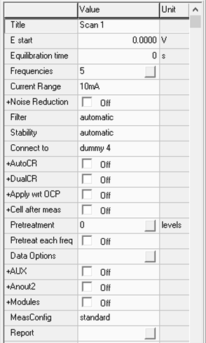
Figure 1: Constant E method parameters.
Note that in the example described here the available settings in Advanced viewing mode are shown. If only the basic settings are required, select Basic viewing mode as described in application note A4.2.
The next step is to define Estart, which in this case is the same as the default value, i.e. 0 V. Similarly, the Equilibration time can be kept at 0 s. Hereafter, the frequency and intervals can be set by pressing the Frequencies button, which opens the Edit frequencies window as shown in Figure 2.
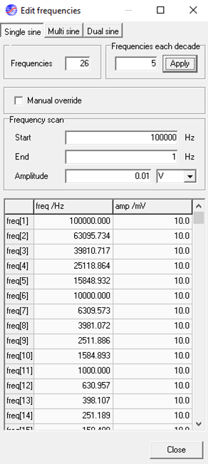
Figure 2: Edit frequencies window.
For the example, the single sine method is used. Multi sine and Dual sine are only interesting if a considerable time advantage can be made and only after comparing the results with single sine to ensure the measurement technique does not negatively impact the results. As an example, a frequency scan between 100,000 Hz to 1 Hz with 5 frequencies each decade and an amplitude of 0.01 V is selected. After pressing the Apply and then the Close button, the Edit frequencies window closes, and the frequencies are added to the method. The current range is fixed at 10 mA. However, as it is common that the impedance of a system can vary over multiple decades it is worthwhile to select AutoCR to automatically select the most accurate current range during the measurement. Noise Reduction, Filter and Stability remain in their default setting. Connect to is set to internal dummy 4, which consists of a 100 Ω resistor (R1) in series with a 1 µF capacitor (C1) parallel over a 1 kΩ resistor (R2) as shown in Figure 3.
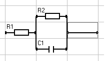
Figure 3: Randles circuit.
This circuit is also known as the Randles circuit and represents the electrolyte resistance (R1), the double layer capacitance (C1) and the charge transfer resistance (R2) of an electrochemical system (see application note A4.3 for more detail). All other settings can remain unchanged.
Start the measurement
The measurement is started by pressing the Start button at the bottom left. The data is updated in real time in the graph during the measurement. With SigView, available from the center of the top bar, the potential and current per frequency are displayed. This is a handy tool to observe how the current responds to the sinusoidal voltage perturbation during the measurement and for post analysis. The Nyquist graph of the completed measurement is depicted in Figure 4, which also shows the SigView window of the central frequency.
Fitting the data
The next step is to fit the data to an equivalent circuit, which can be performed with the Ivium Equivalent Circuit Evaluator that is available from the Analysis dropdown menu.
In this example the equivalent circuit is already known (see Figure 3). Therefore, it can be drawn on the component grid, entered as text string (R1+R2*C1) or as CDC code (R1(R2C1)). The Suggest circuit button will give the same circuit too. Pressing the Fit button will initiate the fitting procedure.
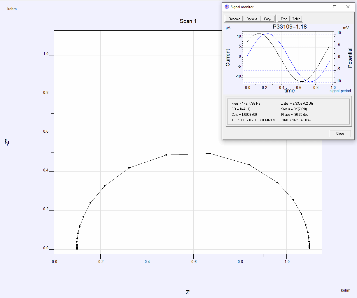
Figure 4: Nyquist graph of Randles circuit. The inset shows the SigView window.
Comparing the fitted values to the actual components confirms that the equivalent circuit indeed matches the measured circuit.

Figure 5: Nyquist graph of Randles circuit. The inset shows the SigView window.
The fit results can be saved to the .idf file by pressing Accept button on the bottom right. Alternatively, the fit data can be saved separately by selecting “Save Fitresult” or “Save as Zplot” which are available from the File dropdown menu in the Ivium Equivalent Circuit Evaluator window. The fit results can be optimized by changing the “Fitting options” available from the “Options” dropdown menu of the top bar of the Ivium Equivalent Circuit Evaluator window. There, it is possible to select which measured parameter should be used to fit best on the theoretical model. Furthermore, the error weight can be adjusted to: