A printable version of this application note is available here: A4.2 – Electrochemical impedance spectroscopy – Setting up a measurement
The EIS measurement is setup in IviumSoft software. Depending on the requirements of the measurement four different impedance methods can be selected from the Method window as shown in Figure 1.
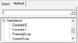
Figure 1: Available impedance methods.
The differences between these methods are:
The first two methods are performed at a fixed potential or current, whereas the last two methods are particularly convenient to quickly get information about the impedance of a system at a different voltage or current. Once a specific potential or current is of interest is identified a more detailed measurement can be performed.
Constant E
Basic mode
By selecting Constant E the method parameters are shown (see Figure 2). Note that these are the method parameters available in Basic mode. If desired a title of measurement can be given. E start is the constant potential that is applied throughout the EIS measurement. The frequency scan be defined by clicking on the box, which opens up the Edit frequencies popup window as shown in Figure 3.
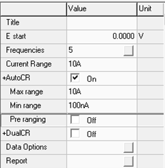
Figure 2: Constant E method parameters in Basic mode.
In the popup window the number of frequencies that will be applied is automatically calculated from the input. The number of frequencies to be applied per decade can be entered on the top right. After selecting Apply, a logarithmic spread of the frequencies will be automatically calculated and listed in the table below. More frequencies mean more data points, but also a longer measurement time, especially at low frequencies.
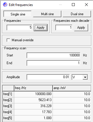
Figure 3: Edit frequencies window.
The start and end frequency can be entered in the corresponding cells. Also, the amplitude of the potential perturbation can be entered. Manual override can be checked, which allows to manually change the individual frequencies and amplitudes in the table below. The latter can be used to create a completely flexible frequency scan. Closing the popup window will apply the frequency settings during the EIS measurement.
Besides single sine the Edit frequencies window offers more advanced sine wave perturbations. These can be selected by the tabs at the top of the window. Multi sine applies multiple sine wave frequencies simultaneously and the corresponding impedances are collected in a single measurement. This is especially useful for measurements at lower frequencies as this can decrease the measurement time considerably and minimize artefacts caused by time-variable impedances. With dual sine a sum of 2 frequencies is applied: 2x and 5x the base frequency. Applying such a signal on a non-linear cell will result in a mix of well-defined modulation products.
The next method parameter in Figure 2 is selecting a fixed current range. A dropdown selection is available by checking the AutoCR box, which overrides the fixed current range, i.e. the instrument will automatically select the most appropriate current range for the measured signal. It is highly recommended to select AutoCR as the potential perturbation during the EIS measurement crosses zero, therefore the current will often change over multiple orders of magnitude.
Selecting the checkbox of Pre ranging enables the automatic current ranging to start before the measurement so that the instrument will automatically look for the best current range setting to start the measurement.
The DualCR option may be checked for potentiostatic frequency scans that use AutoCR. It will override the automatic current range selection and set the current range depending on a user specified frequency:
Note that this option is only active if the AutoCR option is checked.
Advanced mode
In Advanced mode more method parameters can be set. A screenshot of the method window is depicted in Figure 4.
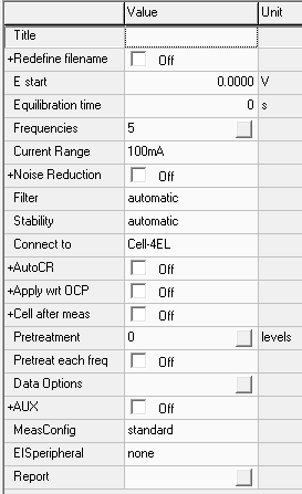
Figure 4: Constant E method parameters in Advanced mode.
The additional parameters are the Equilibration time, which is the time that the E start potential is applied prior to the EIS measurement. Noise reduction can be convenient in cases that suffer from excessive noise. However, it should be used with caution. It has three functions:
When setting up a new method file the Filter and Stability options are set to automatic. In this mode, the system determines the most appropriate setting from the applied frequency. Overriding the automatic setting should be done with care, because it may result in signal deformation. If required it is possible to select the filter to 1 MHz, 100 kHz, 10 kHz, 1 kHz or 10 Hz.
The stability setting determines the bandwidth of the applied signals on the sample: automatic, highspeed, standard or high stability. The bandwidth determines the speed of the control loop of the potentiostat. At higher speed, corrections are applied faster, but the risk of the system becoming instable increases. At lower speed the control loop is slower, and this results in a more stable, but less quickly responsive, system. In automatic mode, the system determines the most appropriate setting from the applied frequency. Overriding the automatic setting should be done with care, because it may result in signal deformation and instability.
With Connect to it is possible to select how the electrochemical cell is connected. Cell-4EL and Cell‑2EL are used for 4 and 2 electrode connections, respectively. Additionally, it is possible to select one of the internal dummy cells, which may be useful to test the method on a known circuit prior to the actual measurement.
Apply wrt OCP can be a convenient way to define the E start or E standby potential versus the open cell potential (OCP).
Constant I
The method parameters of the Constant I impedance technique are almost similar to the Constant E technique. The main difference is that a fixed current range needs to be selected (no AutoCR).
PotentialScan
The implementation is analogue to the Constant E variant, but it is repeated at a range of DC potentials. The start and end potential can be specified as well as the potential step. The results can be stored as single files .idf, or all together as dataset .ids.
CurrentScan
Galvanostatic impedance scans can be performed in combination with a DC current scan, in much the same way as the PotentialScan method. Select the CurrentScan method, and set the DC scan parameters: Istart, Istep and Iend. The frequency scan will now be repeated at every dc-step value of the ramp. The results can be stored as single files .idf, or all together as dataset .ids.
FRA settings
The FRA settings are available by selecting Options>Options from the top ribbon. In the popup window select the corresponding tab. The settings of the stabilization, Results optimization and the acquisition period of the FRA measurement can be adjusted manually, see Figure 5. The default values are sufficient for most measurements; it will not be required to change them. If necessary, the default settings can be reset by selecting the Set default at the bottom of the FRA settings window.
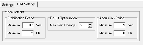
Figure 5: FRA settings options.